Background and proof for Simpson's Rule
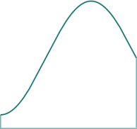
We aim to find the area under the following general curve.
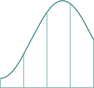
We divide it into 4 equal segments. (It must be an even number of segments for Simpson's Rule to work.)
We next construct parabolas which very nearly match the curve in each of the 4 segments. If we are given 3 points, we can pass a unique parabola through those points.
NOTE: We don't actually need to construct these parabolas when applying Simpson's Rule. This section is just to give you some background on why and how it works.
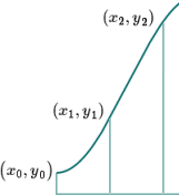
Let's start with the first 2 segments on the left. We take the end points, and the middle point as shown:
We can take measurements (using an overlaid grid) and observe these three points to be:
(x0,y0)=(−1.57,1)
(x1,y1)=(−0.39,1.62)
(x2,y2)=(0.79,2.71)
Using these 3 points, we use the general form of a parabola,
y=ax2+bx+c, and substitute the known
x- and
y-values, as follows.
1=a(−1.57)2+b(−1.57)+c
1.62=a(−0.39)2+b(−0.39)+c
2.71=a(0.79)2+b(0.79)+c
This gives us a set of 3 simultaneous equations in 3 unknowns, which we can solve using
these algebraic methods. Doing so gives us:
a=0.17021, b=0.85820, c=1.92808.
So the parabola passing through those 3 points is
y=0.170x2+0.858x+1.93
Note: Of course, we are using full calculator accuracy throughout, but final results are rounded.
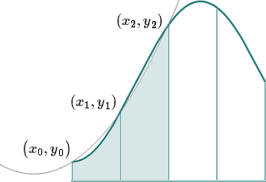
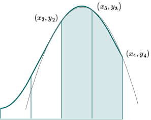
Here is what that parabola looks like:
We can see the parabola passes through the 3 points, and it is close to our original curve, and so it's a good approximation for the curve in that portion of the graph. As usual, the more divisions we take, the more accurate it will be.
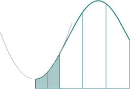
We do the same process for the final 2 segments, and get a parabola that passes through the 3 points shown, and which looks like this:
There are noticeable gaps between the oriignal curve and our parabolas. We only have to halve the segment size to get a much better fit, as we can see in this next image. The parabola is almost identical to the curve.
See an applet that explores this concept here:
Riemann Sums
Proof of Simpson's Rule
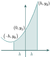
We consider the area under the general parabola
y=ax2+bc+c.
For easier algebra, we start at the point
(0,y1), and consider the area under the parabola between
x=−h and
x=h, as shown. (Note that
Δx=h.)
We have:
∫−hh(ax2+bx+c) dx
=[3ax3+2bx2+cx]−hh
=(3ah3+2bh2+ch)− (−3ah3+2bh2−ch)
=32ah3+2ch
=3h(2ah2+6c) (getting it into a convenient form)
Our parabola passes through
(−h,y0),
(0,y1), and
(h,y2). Substituting these
x- and
y-values into the general equation of our parabola, we get:
y0=ah2−bh+c
y1=c
y2=ah2+bh+c
Solving these gives us
c=y1 (from the second line)
and
2ah2=y0−2y1+y2 (by adding the first and 3rd line)
Substituting these into
A=3h(2ah2+6c) from above, we have:
A=3h(2ah2+6c)
=3h(y0−2y1+y2+6y1)
=3h(y0+4y1+y2)
The parabola passing through the next set of 3 points will have an area of:
A=3h(y2+4y3+y4)
Adding the 2 areas, we get:
A=3h(y0+4y1+2y2+4y3+y4)
Say we have 6 subintervals. We just find the areas under the 3 resulting parabolas, and add them to obtain:
A=3h[y0+4y1+2y2+4y3+ 2y4+ 4y5+ y6]
We could keep going by creating more and more segments, and adding the areas as we go along. and we would obtain Simpson's Rule:
∫abf(x)dx ≈3Δx(y0+4y1+2y2+4y3+ 2y4…+ 4yn−1+ yn)