Saturday 27 July 2019

The Trapezoidal Rule

The Trapezoidal Rule

by M. Bourne

Interactive exploration

See an applet where you can explore Simpson's Rule and other numerical techniques:
Riemann Sums Applet
Problem: Find
\displaystyle{\int_{{0}}^{{1}}}\sqrt{{{x}^{2}+{1}}}\ {\left.{d}{x}\right.}
We put \displaystyle{u}={x}^{2}+{1} then \displaystyle{d}{u}={2}{x}\ {\left.{d}{x}\right.}.
But the question does not contain an `x\ dx` term so we cannot solve it using any of the integration methods we have met so far.
We need to use numerical approaches. (This is usually how software like Mathcad or graphics calculators perform definite integrals).
We can use one of two methods:
  • Trapezoidal rule
  • Simpson's Rule (in the next section: Simpson's Rule)
Continues below 

The Trapezoidal Rule

We saw the basic idea in our first attempt at solving the area under the arches problem earlier.
Instead of using rectangles as we did in the arches problem, we'll use trapezoids (trapeziums) and we'll find that it gives a better approximation to the area.
y0
\displaystyle\Delta{x}
y1
\displaystyle\Delta{x}
y2
\displaystyle\Delta{x}
y3
\displaystyle\Delta{x}
y4
\displaystyle\Delta{x}
y5
\displaystyle\Delta{x}
y6
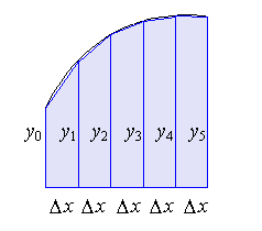
The approximate area under the curve is found by adding the area of all the trapezoids.
(Recall that we write "Δx" to mean "a small change in x".)

Area of a trapezoid

\displaystyle{p}
\displaystyle{q}
\displaystyle{h}
\displaystyle\text{Area}=\frac{h}{{2}}{\left({p}+{q}\right)}
Now, the area of a trapezoid (trapezium) is given by:
\displaystyle\text{Area}=\frac{h}{{2}}{\left({p}+{q}\right)}
We need "right" trapezoids (which means the parallel sides are at right angles to the base), and they are rotated 90° so that their new base is actually h, as follows, and h = Δx.
y0
y1
\displaystyle\Delta{x}
A "typical" trapezoid
So the total area is given by:
\displaystyle\text{Area}\approx\frac{1}{{2}}{\left({y}_{{0}}+{y}_{{1}}\right)}\Delta{x}+ \displaystyle\frac{1}{{2}}{\left({y}_{{1}}+{y}_{{2}}\right)}\Delta{x}+ \displaystyle\frac{1}{{2}}{\left({y}_{{2}}+{y}_{{3}}\right)}\Delta{x}+\ldots
We can simplify this to give us the Trapezoidal Rule, for \displaystyle{n} trapezoids:
\displaystyle\text{Area}\approx \displaystyle\Delta{x}{\left(\frac{{{y}_{{0}}}}{{2}}+{y}_{{1}}+{y}_{{2}}+{y}_{{3}}+\right.} \displaystyle{\left.\ldots+\frac{{{y}_{{n}}}}{{2}}\right)}
To find \displaystyle\Delta{x} for the area from \displaystyle{x}={a} to \displaystyle{x}={b}, we use:
\displaystyle\Delta{x}=\frac{{{b}-{a}}}{{n}}
and we also need
\displaystyle{y}_{{0}}= f{{\left({a}\right)}}
\displaystyle{y}_{{1}}= f{{\left({a}+\Delta{x}\right)}}
\displaystyle{y}_{{2}}= f{{\left({a}+{2}\Delta{x}\right)}}
\displaystyle\ldots
\displaystyle{y}_{{n}}= f{{\left({b}\right)}}

Note

  • We get a better approximation if we take more trapezoids [up to a limit!].
  • The more trapezoids we take, \displaystyle\Delta{x} will tend to \displaystyle{0}, that is, \displaystyle\Delta{x}\rightarrow{0}.
  • We can write (if the curve is above the x-axis only between \displaystyle{x}={a} and \displaystyle{x}={b}):
\displaystyle\text{Area}={\int_{{a}}^{{b}}} f{{\left({x}\right)}}{\left.{d}{x}\right.}
\displaystyle\approx \displaystyle\Delta{x}{\left(\frac{{{y}_{{0}}}}{{2}}+{y}_{{1}}+{\left.\ldots+\frac{{{y}_{{n}}}}{{2}}\right)}\right.}

Don't miss...

There is an interactive applet where you can explore the Trapezoid Rule, here:

Exercise

Using \displaystyle{n}={5}, approximate the integral:
\displaystyle{\int_{{0}}^{{1}}}\sqrt{{{x}^{2}+{1}}}\ {\left.{d}{x}\right.}
Answer

This is the situation:
square root trapezoidal
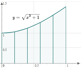
I have joined each of the points at the top of the vertical segments with a straight line.
Here, \displaystyle{a}={0} and \displaystyle{b}={1}, and the width of each trapezoid is given by:
\displaystyle\Delta{x}={\frac{{{b}-{a}}}{{{n}}}}={\frac{{{1}-{0}}}{{{5}}}}={0.2}
\displaystyle{y}_{{0}}= f{{\left({a}\right)}}= \displaystyle f{{\left({0}\right)}}=\sqrt{{{0}^{2}+{1}}}={1}
\displaystyle{y}_{{1}}= f{{\left({a}+\Delta{x}\right)}}= \displaystyle f{{\left({0.2}\right)}}=\sqrt{{{0.2}^{2}+{1}}}={1.0198039}
\displaystyle{y}_{{2}}= f{{\left({a}+{2}\Delta{x}\right)}}= \displaystyle f{{\left({0.4}\right)}}=\sqrt{{{0.4}^{2}+{1}}}={1.0770330}
\displaystyle{y}_{{3}}= f{{\left({a}+{3}\Delta{x}\right)}}= \displaystyle f{{\left({0.6}\right)}}=\sqrt{{{0.6}^{2}+{1}}}={1.1661904}
\displaystyle{y}_{{4}}= f{{\left({a}+{4}\Delta{x}\right)}}= \displaystyle f{{\left({0.8}\right)}}=\sqrt{{{0.8}^{2}+{1}}}={1.2806248}
\displaystyle{y}_{{5}}= f{{\left({a}+{5}\Delta{x}\right)}}= \displaystyle f{{\left({1.0}\right)}}=\sqrt{{{1}^{2}+{1}}}={1.4142136}
So we have:
\displaystyle\text{Integral}\approx
\displaystyle{0.2}{\left(\frac{1}{{2}}\times{1}+{1.0198039}\right.} \displaystyle+{1.0770330}+{1.1661904} \displaystyle{\left.+{1.2806248}+\frac{1}{{2}}\times{1.4142136}\right)}
\displaystyle={1.150}
So \displaystyle{\int_{{0}}^{{1}}}\sqrt{{{x}^{2}+{1}}}\ {\left.{d}{x}\right.}\approx{1.150}
We can see in the graph above the trapezoids are very close to the original curve, so our approximation should be close to the real value. In fact, to 3 decimal places, the integral value is 1.148.