Lesson Note On Solving plane triangles

Solving plane trianglesEdit

Standard notation for a triangle

A general form triangle has six main characteristics (see picture): three linear (side lengths a, b, c) and three angular (α, β, γ). The classical plane trigonometry problem is to specify three of the six characteristics and determine the other three. A triangle can be uniquely determined in this sense when given any of the following:

• Three sides (SSS)
• Two sides and the included angle (SAS)
• Two sides and an angle not included between them (SSA), if the side length adjacent to the angle is shorter than the other side length.
• A side and the two angles adjacent to it (ASA)
• A side, the angle opposite to it and an angle adjacent to it (AAS).
• Three angles (AAA) on the sphere (but not in the plane).

For all cases in the plane, at least one of the side lengths must be specified.

 If only the angles are given, the side lengths cannot be determined, because any similar triangle is a solution

Trigonomic relations

The standard method of solving the problem is to use fundamental relations.

Law of cosines

${\displaystyle a^{2}=b^{2}+c^{2}-2bc\cos \alpha }$

${\displaystyle b^{2}=a^{2}+c^{2}-2ac\cos \beta }$

${\displaystyle c^{2}=a^{2}+b^{2}-2ab\cos \gamma }$

Law of sines

${\displaystyle {\frac {a}{\sin \alpha }}={\frac {b}{\sin \beta }}={\frac {c}{\sin \gamma }}}$

Sum of angles

${\displaystyle \alpha +\beta +\gamma =180^{\circ }}$

Law of tangents

${\displaystyle {\frac {a-b}{a+b}}={\frac {\tan[{\frac {1}{2}}(\alpha -\beta )]}{\tan[{\frac {1}{2}}(\alpha +\beta )]}}.}$

There are other (sometimes practically useful) universal relations:

 the law of cotangents and Mollweide's formula.

NotesEdit

1. To find an unknown angle, the law of cosines is safer than the law of sines. The reason is that the value of sine for the angle of the triangle does not uniquely determine this angle. For example, if sin β = 0.5, the angle β can equal either 30° or 150°. Using the law of cosines avoids this problem: within the interval from 0° to 180° the cosine value unambiguously determines its angle. On the other hand, if the angle is small (or close to 180°), then it is more robust numerically to determine it from its sine than its cosine because the arc-cosine function has a divergent derivative at 1 (or −1).
2. We assume that the relative position of specified characteristics is known. If not, the mirror reflection of the triangle will also be a solution. For example, three side lengths uniquely define either a triangle or its reflection.

Three sides given (SSS)Edit

Three sides given

Let three side lengths a, b, c be specified. To find the angles α, β, the law of cosines can be used:

${\displaystyle {\begin{aligned}\alpha &=\arccos {\frac {b^{2}+c^{2}-a^{2}}{2bc}}\\[4pt]\beta &=\arccos {\frac {a^{2}+c^{2}-b^{2}}{2ac}}.\end{aligned}}}$

Then angle γ = 180° − α − β.

Some sources recommend to find angle β from the law of sines but (as Note 1 above states) there is a risk of confusing an acute angle value with an obtuse one.

Another method of calculating the angles from known sides is to apply the law of cotangents.

Two sides and the included angle given (SAS)Edit

Two sides and the included angle given

Here the lengths of sides a, b and the angle γ between these sides are known. The third side can be determined from the law of cosines:

${\displaystyle c={\sqrt {a^{2}+b^{2}-2ab\cos \gamma }}.}$

Now we use law of cosines to find the second angle:

${\displaystyle \alpha =\arccos {\frac {b^{2}+c^{2}-a^{2}}{2bc}}.}$

Finally, β = 180° − α − γ.

Two sides and non-included angle given (SSA)Edit

Two sides and a non-included angle given

Two solutions for the triangle

This case is not solvable in all cases; a solution is guaranteed to be unique only if the side length adjacent to the angle is shorter than the other side length. Assume that two sides b, c and the angle β are known. The equation for the angle γ can be implied from the law of sines:

${\displaystyle \sin \gamma ={\frac {c}{b}}\sin \beta .}$

We denote further D = c/b sin β (the equation's right side). There are four possible cases:

1. If D > 1, no such triangle exists because the side b does not reach line BC. For the same reason a solution does not exist if the angle β ≥ 90° and b ≤ c.
2. If D = 1, a unique solution exists: γ = 90°, i.e., the triangle is right-angled.
3. If D < 1 two alternatives are possible.
   1. If b ≥ c, then β ≥ γ (the larger side corresponds to a larger angle). Since no triangle can have two obtuse angles, γ is an acute angle and the solution γ = arcsin D is unique.
   2. If b < c, the angle γ may be acute: γ = arcsin D or obtuse: γ′ = 180° - γ. The figure on right shows the point C, the side b and the angle γ as the first solution, and the point C′, side b′ and the angle γ′ as the second solution.

Once γ is obtained, the third angle α = 180° − β − γ.

The third side can then be found from the law of sines:

${\displaystyle a=b\ {\frac {\sin \alpha }{\sin \beta }}}$

or

${\displaystyle a=c\cos \beta \pm {\sqrt {b^{2}-c^{2}\sin ^{2}\beta }}}$

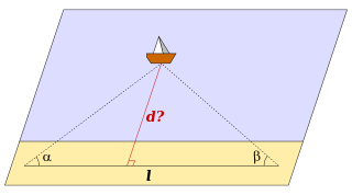
A side and two adjacent angles given (ASA)Edit

One side and two adjacent angles given

The known characteristics are the side c and the angles α, β. The third angle γ = 180° − α − β.

Two unknown side can be calculated from the law of sines:

${\displaystyle a=c\ {\frac {\sin \alpha }{\sin \gamma }};\quad b=c\ {\frac {\sin \beta }{\sin \gamma }}.}$

or

${\displaystyle a=c{\frac {\sin \alpha }{\sin \alpha \cos \beta +\sin \beta \cos \alpha }}}$

${\displaystyle b=c{\frac {\sin \beta }{\sin \alpha \cos \beta +\sin \beta \cos \alpha }}}$

Lesson Note On Solving the least squares problem

Solving the least squares problemEdit

The minimum of the sum of squares is found by setting the gradient to zero. 

Since the model contains m parameters, there are m gradient equations:

${\displaystyle {\frac {\partial S}{\partial \beta _{j}}}=2\sum _{i}r_{i}{\frac {\partial r_{i}}{\partial \beta _{j}}}=0,\ j=1,\ldots ,m,}$

and since ${\displaystyle r_{i}=y_{i}-f(x_{i},{\boldsymbol {\beta }})}$, the gradient equations become

${\displaystyle -2\sum _{i}r_{i}{\frac {\partial f(x_{i},{\boldsymbol {\beta }})}{\partial \beta _{j}}}=0,\ j=1,\ldots ,m.}$

The gradient equations apply to all least squares problems. 

Each particular problem requires particular expressions for the model and 

its partial derivatives.

Linear least squaresEdit

A regression model is a linear one when the model comprises a linear combination 

of the parameters, i.e.,

${\displaystyle f(x,\beta )=\sum _{j=1}^{m}\beta _{j}\phi _{j}(x),}$

where the function ${\displaystyle \phi _{j}}$ is a function of ${\displaystyle x}$.

Letting

${\displaystyle X_{ij}={\frac {\partial f(x_{i},{\boldsymbol {\beta }})}{\partial \beta _{j}}}=\phi _{j}(x_{i}),}$

we can then see that in that case the least square estimate (or estimator, 

in the context of a random sample), ${\displaystyle {\boldsymbol {\beta }}}$ is given by

${\displaystyle {\boldsymbol {\hat {\beta }}}=(X^{T}X)^{-1}X^{T}{\boldsymbol {y}}.}$

For a derivation of this estimate see Linear least squares (mathematics).

Non-linear least squaresEdit

There is, in some cases, a closed-form solution to a non-linear least squares problem – 

but in general there is not. In the case of no closed-form solution, numerical algorithms 

are used to find the value of the parameters ${\displaystyle \beta }$ that minimizes the objective. 

Most algorithms involve choosing initial values for the parameters. Then, 

the parameters are refined iteratively, that is, the values are obtained by successive 

approximation:

${\displaystyle {\beta _{j}}^{k+1}={\beta _{j}}^{k}+\Delta \beta _{j},}$

where a superscript k is an iteration number, and the vector of increments ${\displaystyle \Delta \beta _{j}}$ 

is called the shift vector. In some commonly used algorithms, at each iteration the 

model may be linearized by approximation to a first-order Taylor series expansion

 about ${\displaystyle {\boldsymbol {\beta }}^{k}}$:

${\displaystyle {\begin{aligned}f(x_{i},{\boldsymbol {\beta }})&=f^{k}(x_{i},{\boldsymbol {\beta }})+\sum _{j}{\frac {\partial f(x_{i},{\boldsymbol {\beta }})}{\partial \beta _{j}}}\left(\beta _{j}-{\beta _{j}}^{k}\right)\\&=f^{k}(x_{i},{\boldsymbol {\beta }})+\sum _{j}J_{ij}\,\Delta \beta _{j}.\end{aligned}}}$

The Jacobian J is a function of constants, the independent variable and the parameters, 

so it changes from one iteration to the next. The residuals are given by

${\displaystyle r_{i}=y_{i}-f^{k}(x_{i},{\boldsymbol {\beta }})-\sum _{k=1}^{m}J_{ik}\,\Delta \beta _{k}=\Delta y_{i}-\sum _{j=1}^{m}J_{ij}\,\Delta \beta _{j}.}$

To minimize the sum of squares of ${\displaystyle r_{i}}$, the gradient equation is set to zero and solved for

 ${\displaystyle \Delta \beta _{j}}$:

${\displaystyle -2\sum _{i=1}^{n}J_{ij}\left(\Delta y_{i}-\sum _{k=1}^{m}J_{ik}\,\Delta \beta _{k}\right)=0,}$

which, on rearrangement, become m simultaneous linear equations, 

the normal equations:

${\displaystyle \sum _{i=1}^{n}\sum _{k=1}^{m}J_{ij}J_{ik}\,\Delta \beta _{k}=\sum _{i=1}^{n}J_{ij}\,\Delta y_{i}\qquad (j=1,\ldots ,m).}$

The normal equations are written in matrix notation as

${\displaystyle \mathbf {(J^{T}J)\,\Delta {\boldsymbol {\beta }}=J^{T}\,\Delta y} .\,}$

These are the defining equations of the Gauss–Newton algorithm.

Solving spherical triangles

Solving spherical triangles Edit The general spherical triangle is fully determined by three of its six characteristics (3 sides and 3 angles). Note that the sides a, b, c of a spherical triangle are measured by angular rather than linear units, based on the corresponding central angles. The solution of triangles for non-Euclidean spherical geometry has some differences from the planar case. For example, the sum of the three angles α + β + γ depends on the triangle. In addition, there are no unequal similar triangles, and so the problem of constructing a triangle with specified three angles has a unique solution. The basic relations used to solve a problem are similar to those of the planar case: see Law of cosines (spherical) and Law of sines (spherical). Among other relationships that may be useful are the half-side formula and Napier's analogies:[7] {\displaystyle \tan {\frac {c}{2}}\cos {\frac {\alpha -\beta }{2}}=\tan {\frac {a+b}{2}}\cos {\frac {\alpha +\beta }{2}}} {\displaystyle \tan {\frac {c}{2}}\sin {\frac {\alpha -\beta }{2}}=\tan {\frac {a-b}{2}}\sin {\frac {\alpha +\beta }{2}}} {\displaystyle \cot {\frac {\gamma }{2}}\cos {\frac {a-b}{2}}=\tan {\frac {\alpha +\beta }{2}}\cos {\frac {a+b}{2}}} {\displaystyle \cot {\frac {\gamma }{2}}\sin {\frac {a-b}{2}}=\tan {\frac {\alpha -\beta }{2}}\sin {\frac {a+b}{2}}.}  Three sides given Three sides given (spherical SSS) Edit Known: the sides a, b, c (in angular units). The triangle's angles are computed from the spherical law of cosines: {\displaystyle \alpha =\arccos \left({\frac {\cos a-\cos b\ \cos c}{\sin b\ \sin c}}\right),} {\displaystyle \beta =\arccos \left({\frac {\cos b-\cos c\ \cos a}{\sin c\ \sin a}}\right),} {\displaystyle \gamma =\arccos \left({\frac {\cos c-\cos a\ \cos b}{\sin a\ \sin b}}\right).}  Two sides and the included angle given Two sides and the included angle given (spherical SAS) Edit Known: the sides a, b and the angle γ between them. The side c can be found from the law of cosines: {\displaystyle c=\arccos \left(\cos a\cos b+\sin a\sin b\cos \gamma \right).} The angles α', β can be calculated as above, or by using Napier's analogies: {\displaystyle \alpha =\arctan \ {\frac {2\sin a}{\tan({\frac {\gamma }{2}})\sin(b+a)+\cot({\frac {\gamma }{2}})\sin(b-a)}},} {\displaystyle \beta =\arctan \ {\frac {2\sin b}{\tan({\frac {\gamma }{2}})\sin(a+b)+\cot({\frac {\gamma }{2}})\sin(a-b)}}.} This problem arises in the navigation problem of finding the great circle between two points on the earth specified by their latitude and longitude; in this application, it is important to use formulas which are not susceptible to round-off errors. For this purpose, the following formulas (which may be derived using vector algebra) can be used: {\displaystyle {\begin{aligned}c&=\arctan {\frac {\sqrt {(\sin a\cos b-\cos a\sin b\cos \gamma )^{2}+(\sin b\sin \gamma )^{2}}}{\cos a\cos b+\sin a\sin b\cos \gamma }},\\\alpha &=\arctan {\frac {\sin a\sin \gamma }{\sin b\cos a-\cos b\sin a\cos \gamma }},\\\beta &=\arctan {\frac {\sin b\sin \gamma }{\sin a\cos b-\cos a\sin b\cos \gamma }},\end{aligned}}} where the signs of the numerators and denominators in these expressions should be used to determine the quadrant of the arctangent.  Two sides and a non-included angle given Two sides and non-included angle given (spherical SSA) Edit This problem is not solvable in all cases; a solution is guaranteed to be unique only if the side length adjacent to the angle is shorter than the other side length. Known: the sides b, c and the angle β not between them. A solution exists if the following condition holds: {\displaystyle b>\arcsin(\sin c\,\sin \beta ).} The angle γ can be found from the spherical law of sines: {\displaystyle \gamma =\arcsin \left({\frac {\sin c\,\sin \beta }{\sin b}}\right).} As for the plane case, if b < c then there are two solutions: γ and 180° - γ. We can find other characteristics by using Napier's analogies: {\displaystyle a=2\arctan \left[\tan \left({\tfrac {1}{2}}(b-c)\right){\frac {\sin \left({\tfrac {1}{2}}(\beta +\gamma )\right)}{\sin \left({\tfrac {1}{2}}(\beta -\gamma )\right)}}\right],} {\displaystyle \alpha =2\operatorname {arccot} \left[\tan \left({\tfrac {1}{2}}(\beta -\gamma )\right){\frac {\sin \left({\tfrac {1}{2}}(b+c)\right)}{\sin \left({\tfrac {1}{2}}(b-c)\right)}}\right].}  One side and two adjacent angles given A side and two adjacent angles given (spherical ASA) Edit
Three angles given (spherical AAA)Edit

Known: the angles α, β, γ. From the law of cosines we infer:

{\displaystyle a=\arccos \left({\frac {\cos \alpha +\cos \beta \cos \gamma }{\sin \beta \sin \gamma }}\right),}{\displaystyle b=\arccos \left({\frac {\cos \beta +\cos \gamma \cos \alpha }{\sin \gamma \sin \alpha }}\right),}{\displaystyle c=\arccos \left({\frac {\cos \gamma +\cos \alpha \cos \beta }{\sin \alpha \sin \beta }}\right).}

Solving right-angled spherical trianglesEdit

The above algorithms become much simpler if one of the angles of a triangle (for example, the angle C) is the right angle. Such a spherical triangle is fully defined by its two elements, and the other three can be calculated usingNapier's Pentagon or the following relations.

{\displaystyle \sin a=\sin c\cdot \sin A} (from the Law of sines (spherical)){\displaystyle \tan a=\sin b\cdot \tan A}{\displaystyle \cos c=\cos a\cdot \cos b} (from the law of cosines (spherical)){\displaystyle \tan b=\tan c\cdot \cos A}{\displaystyle \cos A=\cos a\cdot \sin B} (also from the law of cosines){\displaystyle \cos c=\cot A\cdot \cot B}

Some applicationsEdit

TriangulationEdit

Distance measurement by triangulation

Main article: Triangulation

If one wants to measure the distance dfrom shore to a remote ship via triangulation, one marks on the shore two points with known distance lbetween them (the baseline). Let α, β be the angles between the baseline and the direction to the ship.

From the formulae above (ASA case) one can define the length of the triangle height:

{\displaystyle d={\frac {\sin \alpha \,\sin \beta }{\sin(\alpha +\beta )}}\,l={\frac {\tan \alpha \,\tan \beta }{\tan \alpha +\tan \beta }}\,l.}

This method is used in cabotage. The angles α, β are defined by observation of familiar landmarks from the ship.

How to measure a mountain's height

As another example, if one wants to measure the height h of a mountain or a high building, the angles α, β from two ground points to the top are specified. Let l be the distance between these points. From the same ASA case formulas we obtain:

{\displaystyle h={\frac {\sin \alpha \,\sin \beta }{\sin(\beta -\alpha )}}\,l={\frac {\tan \alpha \,\tan \beta }{\tan \beta -\tan \alpha }}\,l.}

The distance between two points on the globeEdit

Main article: Great-circle distance

To calculate the distance between two points on the globe,

Point A: latitude λ_A, longitude L_A, andPoint B: latitude λ_B, longitude L_B

we consider the spherical triangle ABC, where C is the North Pole. Some characteristics are:

{\displaystyle a=90^{\mathrm {o} }-\lambda _{\mathrm {B} },\,}{\displaystyle b=90^{\mathrm {o} }-\lambda _{\mathrm {A} },\,}{\displaystyle \gamma =L_{\mathrm {A} }-L_{\mathrm {B} }.\,}

If two sides and the included angle given, we obtain from the formulas

{\displaystyle \mathrm {AB} =R\arccos \left[\sin \lambda _{\mathrm {A} }\,\sin \lambda _{\mathrm {B} }+\cos \lambda _{\mathrm {A} }\,\cos \lambda _{\mathrm {B} }\,\cos \left(L_{\mathrm {A} }-L_{\mathrm {B} }\right)\right].}

Here R is the Earth's radius.